The Full MLOps Blueprint: Model Development and Optimization—Part C

Recap

Before we dive into Part 10 of this MLOps and LLMOps crash course, let’s quickly recap what we covered in the previous part.

In Part 9, we discussed model optimization and basic compression techniques.

We started by understanding what fine-tuning is and what a transfer learning plus fine-tuning pipeline looks like.

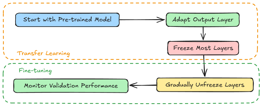
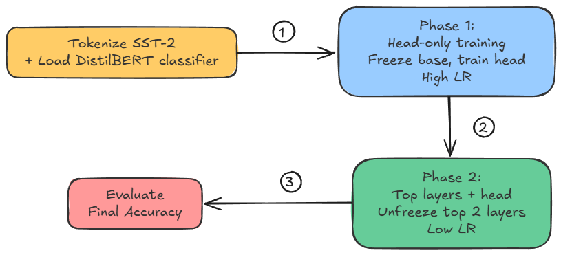
Next, we covered a hands-on example demonstrating transfer learning + fine-tuning in action, on a small, fast BERT variant, distilbert-base-uncased.

From there we dived into model compression. We understood pruning and its type and how exactly it helps us in compression.

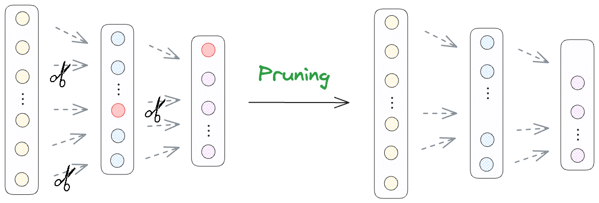
Finally, we also walked through a hands-on demo on unstructured and structured pruning, with prune-finetune alteration for maintained performance.

If you haven’t explored Part 9 yet, we recommend going through it first since it lays the conceptual foundation that’ll help you better understand what we’re about to dive into here.

Read it here:

The Full MLOps Blueprint: Model Development and Optimization—Part B

MLOps and LLMOps Crash Course—Part 9.

Daily Dose of Data ScienceAvi Chawla

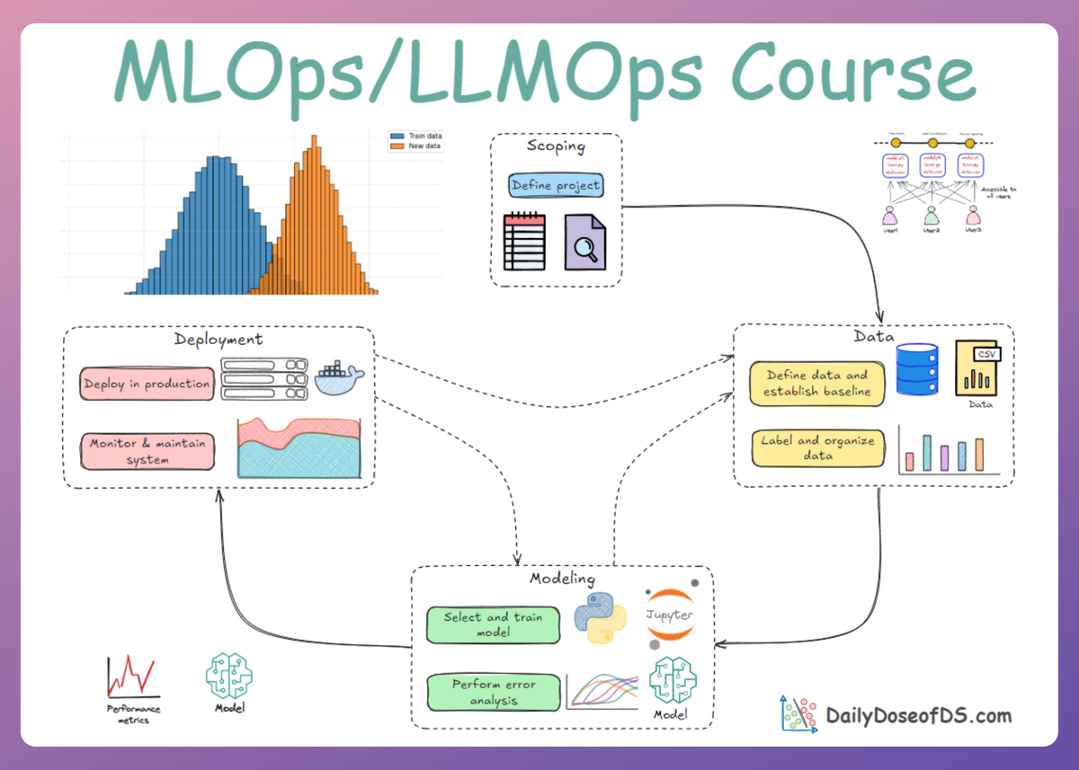
In this chapter, we’ll continue with model compression itself (part of the modeling phase of the ML system lifecycle), diving deep into model compression techniques beyond pruning.

As always, every idea and notion will be backed by concrete examples, walkthroughs, and practical tips to help you master both the idea and the implementation.

Let's begin!

Model compression (contd.)

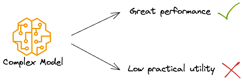
As we already know by now, the models that score highest on accuracy benchmarks are not always the models that make it to production.

They may be too slow or too large. Model compression reduces the computational footprint of a model.

A smaller, faster model is easier to deploy (especially on edge devices or at scale) and often cheaper to run. We already learned about pruning in the previous chapter, and in this chapter, we'll cover:

• Knowledge Distillation
• Low-Rank Factorization
• Quantization

Let's examine each technique in detail, including how they work and possibly some code or pseudocode examples.

Knowledge distillation

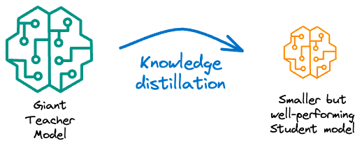
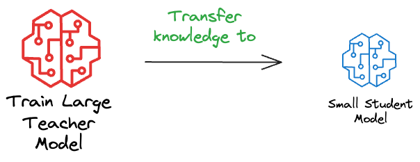
Knowledge Distillation (KD) is a technique where a large, complex model (teacher) transfers its knowledge to a smaller model (student).

The concept is that a small model can be trained not just on the original data labels, but on the soft predictions of the large model, thereby learning to mimic the large model’s function.

Why this works?

The teacher model’s output probabilities often contain richer information than the one-hot labels. For example, if class A is 10 times more likely than class B according to the teacher, that gives the student a hint about class B being the second-best option, etc.

This dark knowledge (as it's called) helps the student learn the teacher’s decision boundaries more faithfully than it would just from ground truth one-hot labels.

There are several benefits to this:

• The student can be much smaller yet achieve performance close to that of the teacher.
• You can distill an ensemble of models into one student (the teacher can be a group of models whose outputs are averaged, and the student learns from that).
• Distillation sometimes even improves accuracy on the student compared to training it normally on the dataset (the teacher acts as a smoother, providing a better training signal).

But of course, some trade-offs are also involved.

You have to train the large teacher model first, which is an upfront cost. In some cases, training the teacher is expensive, but you might already have one (e.g., use an existing public model as a teacher).

Also, the student usually cannot exceed the teacher’s accuracy (there are some cases in which it might, if the teacher’s knowledge helps generalization, but generally, the teacher is typically the upper bound).

Moreover, in a resource-constrained environment, it may not be feasible to train a large teacher model in the first place.

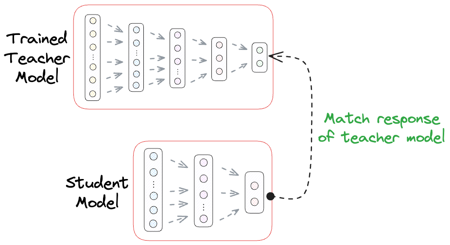
Assuming we are not resource-constrained, at least in the development environment, one of the most common techniques for Knowledge Distillation is Response-based Knowledge Distillation.

As the name suggests, in response-based knowledge distillation, the focus is on matching the output responses (predictions) of the teacher model and the student model.

Workflow pipeline

• Train the teacher model on your training data (standard training).
• Freeze the teacher (or keep it fixed) and train the student model. The student’s training objective is a combination of:
  • A standard loss against the true labels (e.g., cross-entropy with ground truth). This ensures the student still learns the actual task.
  • A distillation loss that makes the student’s output distribution match the teacher’s output distribution. Typically, this is done with the Kullback-Leibler divergence (KL divergence) between the softmax outputs of teacher and student.
• Often, the teacher’s softmax outputs are taken at a higher "temperature". The idea of temperature in distillation is to soften the probability distribution (the teacher might be very confident in one class, which gives almost 0/1 probabilities; by using a temperature > 1 in softmax, we get a softer distribution that retains the rank of confidences but not as peaked). The student also uses the same temperature in its softmax for the loss calculation. This is a detail, but it helps learning.

Quick note for those who might not know:

KL divergence between two probability distributions P(x) and Q(x) is calculated as follows:

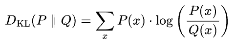
The formula for KL divergence can be read as follows:

The KL divergence between two probability distributions P and Q is calculated by summing the above quantity over all possible outcomes x. Here:

• P(x) represents the probability of outcome x occurring according to distribution P.
• Q(x) represents the probability of the same outcome occurring according to distribution Q.

It measures how much information is lost when using distribution Q to approximate distribution P.

Imagine this. Say P and Q were identical. This should result in zero loss of information.

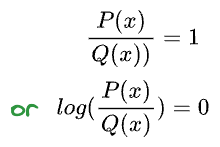
And, hence:

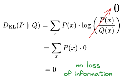
Thus, the more information is lost, the greater the KL divergence. As a result, the more the dissimilarity.

Let's outline the code for knowledge distillation using PyTorch as an example.

We will use MNIST (a relatively small dataset) to demonstrate, with a larger "teacher" model (like a CNN) and a smaller "student" model (like a simple feedforward network).

Find the notebook attached below: